I saw this use case in one of the challenge labs from Google skillboost, and it kind of intrigued me, so I decided to reproduce it.
It’s quite easy to export historic data and ratings from Financial Modeling Prep for a certain stock. In my case that was Merck, a drug producer.
So, I quickly drafted the following script:
import requests
import os
import json
import time
FMP_KEY = os.getenv("FMP_KEY")
symbol = input("Enter stock symbol: ").upper()
start_date = input("Enter start date (YYYY-MM-DD): ")
end_date = input("Enter end date (YYYY-MM-DD): ")
url = f"https://financialmodelingprep.com/stable/historical-price-eod/full?symbol={symbol}&from={start_date}&to={end_date}&apikey={FMP_KEY}"
def fetch_json(url):
try:
response = requests.get(url)
response.raise_for_status() # Raise an error for bad status codes
return response.json()
except requests.exceptions.RequestException as e:
print(f"An error occurred: {e}")
return None
data = fetch_json(url)
with open(f"{symbol}_historical_data.json", "w") as f:
for item in data:
f.write(json.dumps(item) + "\n")
date_format = "%Y-%m-%d"
t1 = time.mktime(time.strptime(start_date, date_format))
t2 = time.mktime(time.strptime(end_date, date_format))
days = int((t2 - t1) / 86400)
url_rating=f"https://financialmodelingprep.com/stable/ratings-historical?symbol={symbol}&limit={days}&apikey={FMP_KEY}"
data_rating = fetch_json(url_rating)
with open(f"{symbol}_historical_ratings.json", "w") as f:
for item in data_rating:
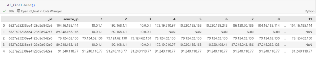
f.write(json.dumps(item) + "\n")This script creates two New Line Delimiter JSON (which actually means that each JSON entry is a completely independent JSON on a line, and this is the BigQuery format supported for Schema Recognition)
After the files are exported, I manually created two tables from these files called mkr_ratings and mrk_historical
Good, now we have to denormalize some of the data and add our RECORD struct between the tables.
Not wanting to waste time, I added the schema from GUI like
[
{
"name": "price",
"type": "RECORD",
"mode": "NULLABLE",
"fields": [
{
"name": "close",
"type": "FLOAT",
"mode": "NULLABLE"
},
{
"name": "spread",
"type": "FLOAT",
"mode": "NULLABLE"
},
{
"name": "change",
"type": "FLOAT",
"mode": "NULLABLE"
}
]
}
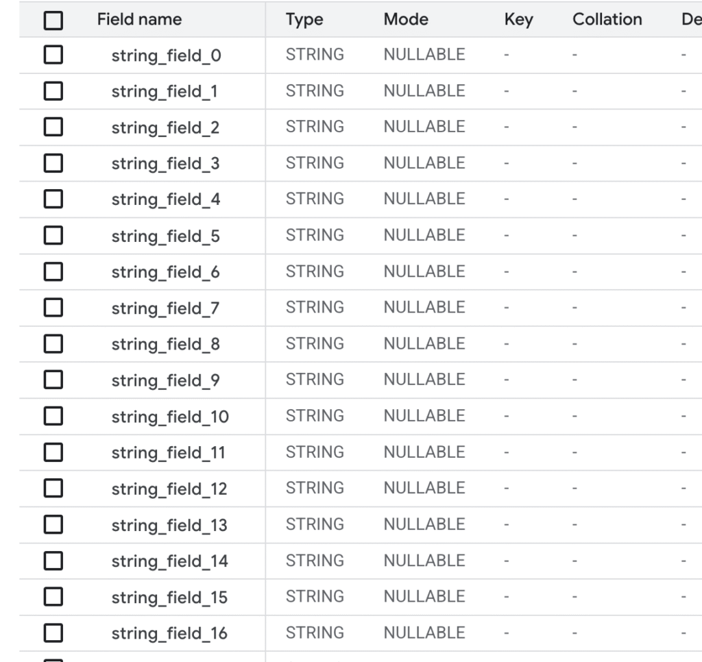
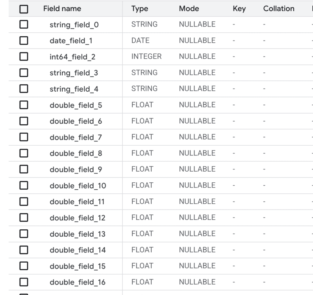
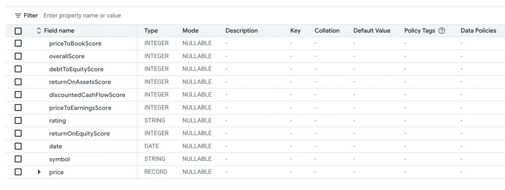
]In the end the schemas looked like this:
mkr_historical
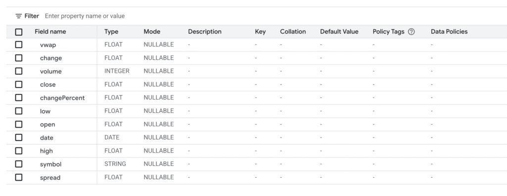
mkr_ratings
And now we need to map data from historical to ratings in the following relation.
mrk_historical.close AS price.close
mrk_historical.spread AS price.spread
mrk_historical.change AS price.change
We also need a anchor field and that is in our case date, which is present in both tables.
After trying to draft it by myself and review it and improve it using a little bit of LLM help, I reached the following form, which is annoyingly simple.
UPDATE `[GCP_PROJECT]`.smallcaps.mrk_ratings AS mrk_ratings
SET
  price = STRUCT(mrk_historical.close AS close, mrk_historical.spread AS spread, mrk_historical.change AS change)
FROM
  `[GCP_PROJECT]`.smallcaps.mrk_historical AS mrk_historical
WHERE
  mrk_ratings.date = mrk_historical.date;
So, you just update the first table and give it an alias, set the actual RECORD as a STRUCT of the required fields from the second table, and at the end match the anchor column of both aliases. Sweet!